The graph created in MS Excel demonstrates the MTV for rolling changes in the pipeline. It is possible to locate the places where it changes significantly and to calculate how much velocity is required to transport particles at specific sections along the pipeline route. The pipeline angle and flow regime are factors that influence the MTV.
 |
To perform the analysis, engineers modeled the fluid flow in a production system and identified places of flow-pattern transition. A commercial software, called PROSPER, was used to obtain data input parameters for the production system, such as pipework length, dimensions, angles and find fluid properties, pressure and temperature profiles using appropriate correlations. The software contains several examples of subsea wells and one of them (subsea black oil well, 11,400ft subsea true vertical depth, 10mi-long subsea flowline) was taken for this project.
PVT data and nodal pressures (well head pressure (WHP), pressure at the manifold) were assumed and the software calculated the bottomhole pressure from the WHP under the specified operating conditions (5000 STB/d). Hence, the pressure traverse curves were generated for the tubing and flowline and correlation comparison was performed. The Beggs and Brill (1973) correlation showed the best closeness of fit and was chosen for the flow pattern identification.
After the software has specified which flow patterns prevail in the production system, the project moved to the second phase – creation of the analytical model in MS Excel with the main objective of finding places of solid phase deposition. The solid phase loading and dimensions were assumed, specifying the flow as diluted with spherical particles. The fluid flow parameters were transferred onto the Excel spreadsheet for calculations, which started with plotting fluid flow velocity field profiles for different flow regimes. In order to do this, the pipeline diameter was divided in five segments on each side from the pipe center and the fluid velocity was found at each of them.
With the velocity profiles thus generated it became clear how quickly the fluid moves in the production system. The next step was to find the minimum transport velocity at which particles would roll and be transported in suspended mode. Obviously, if somewhere in the pipeline the lowest barrier for transport (MTV for rolling) is not met by the actual fluid velocity it means that particles will deposit on the pipeline wall. Therefore, the comparison between the two velocities was done and showed that the condition for solids transport was not satisfied only in the vertical section of the wellbore.
The higher barrier (MTV for suspension) was also found and compared with the actual flow velocities. The comparison showed that although the condition for transport was satisfied in most of the pipeline, particles were rolling alongside of the wall. Only in the horizontal section of the pipeline and close to the manifold the solid phase was transported in suspension. It is important to note that the safest method of the solid phase transport is in suspension, as when particles roll there is the possibility of deposition as pressure drops further down the pipeline.
In places of deposition, the severity of blockage is determined by the height of the deposited bed, which can show the degree of production impairment. In this project it was attempted to analytically derive it from the given equations. Evidently, the top of the deposited bed is at the point where transport occurs, in other words, where the actual flow velocity is equal to MTV for rolling. Thus, the two equations were equalized and the distance from the pipe center where transport occurs was expressed. It then became possible to find the height of the bed by subtracting this distance from the rest of the pipe diameter space. The method proved to be reliable and demonstrated only small error margin (<0.5 %).
The project has laid the ground work for further development and industrial application. Apart from enabling location of places of deposition in the pipeline, it has given the insight into the key relationships between flow parameters and the solid deposition behavior as well as severity of blockage. The next step for this model will be its application in a field case study and comparisons of results with a real-time data. There is the opportunity to further complicate the model by adding parameters close to a real case scenario (non-spherical particles, paraffin, hydrates and wax occurrence, dense flow, varying operating conditions).
On demonstrating the reliability of this model and acknowledging its practical importance it would be possible to incorporate it into an industrial software. Thus, it would be a useful tool in the production engineer’s hands for predicting solid deposition behavior in the production system under varying operating conditions. Subsequently, it might act as a part of an integrated subsea tieback flow assurance management strategy.
 Subscribe